
It is a truth universally acknowledged that internet service providers wish to be invisible to their customers. After all, internet access should be something that works without interruption and doesn’t require intervention. When it does, it becomes a source of frustration for the customer and extra work for the provider.
The way that internet service providers attempt to solve customer problems is through call centers. However, these are a major source of costs, which is why providers are always on the lookout for solutions that will help them optimize their operations. Ideally, problem-solving would be entirely automated with the right software, so that the customers wouldn’t need to call support altogether. Alternatively, the software should help support technicians to solve the problem faster by identifying its source or providing known solutions.
Recently, we decided to investigate how machine learning could help with that. This was made possible by the access we had to a large data set from one of the Broadband Service Assurance Platform’s telco clients which we could analyze in depth. The set consisted of both network data, i.e. metrics on physical characteristics of wired connection to customer premises, as well as business data, i.e. a corresponding list of all support calls customers made. Having these two data sources, we wanted to analyze if we could predict customer problems (support calls) based on the characteristics presented by their wired connection (line data). As long as some subset of problems was caused by the physical layer, this seemed reasonable.
Assuming that we could predict problems based on the line data, what would be the use? We identified four main benefits to that.
- First, quite obviously, this would give the support technicians information about customer problems before these were actually reported.
- If the analysis showed that the problem might be related to some physical characteristics of the connection, we could show this information to the technician, helping them identify the issue and troubleshoot it faster. This would both prove that the problem is real (it is not invalid) and that it is related to the physical layer and not, for example, configuration issues.
- We could also point to specific features on the charts that suggest problems or point to a specific subclass of problems. This would also be helpful in troubleshooting; however, it would require our model to be explainable, i.e. we’d need to be able to know how it arrived at its conclusions.
- Finally, if we could pinpoint specific issues (and not just problematic areas), it would allow us to perform automatic fixes in the next step.
The solution could therefore potentially benefit our telco customers at two different points: before the customer calls (by enabling auto-healing) or if this fails, after they call (by helping the technicians arrive at the right diagnosis and solve the problem faster).
The data
We had access to two main sources of data: wired connection quality measurements and support tickets filed by the customer care engineers.
Wired connection quality is measured between the end user’s device and the telephone exchange. The parameters measured include various physical signal characteristics and transmission errors (see table below). The connection can be established over a phone line (DSL) or a TV cable (HFC). The data is collected by a device management platform, such as AVSystem’s Unified Management Platform, from telco’s equipment (DSLAMs or CMTSes). Then it is sent to the Broadband Service Assurance Platform, which processes it and presents it to the customer care engineers.
The second source of data was support tickets. These were the source of information that at a specific point in time a customer reported a problem with a particular device.
| Available on | ||||
|---|---|---|---|---|
| Parameter | DSL | HFC | Bidirectional | Description |
| SNR | Y | Y | Y | signal to noise ratio, measured in decibels |
| Attenuation | Y | Y | Y | how much electrical signal is lost along the cable |
| Power | Y | Y | Y | transmission power |
| FEC, HEC, CRC | Y | N | Y | various kinds of transmission errors |
| Link retrain | Y | N | N | number of times the connection had to be reestablished |
| Registration status | N | Y | N | status of the connection – normally this should be “connected” or “disconnected,” other states (like “connecting” for an extended time) may signal problems |
| QoS | Y | N | N | reported quality of service |
| Operational status | Y | Y | N | whether the line is up or down |
| Current technology | Y | Y | N | specific connection protocol – whether it's ADSL or ADSL+, or DOCSIS version |
Data analysis
Before doing any modeling, it is always advisable to first look at the data and see what it actually contains. This is to check for patterns that are visible to the naked eye and see whether data requires any cleanup. The first thing to do was to just plot the parameters over time for a sample of lines.
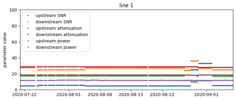
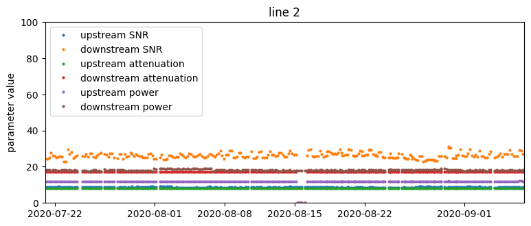
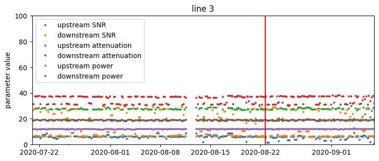
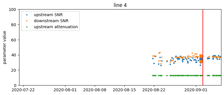
Time series of SNR, attenuation, and transmit power parameter values from four selected lines. The red vertical line is the occurrence of a support ticket.
Based on just that, we could make some observations:
- There are no visually obvious patterns in connection parameters that could forecast support calls. This suggests that the problem is not trivial and we should approach it using machine learning methods.
- There is great heterogeneity with respect to the variability of measurements – the same parameter can vary considerably on one device and be constant on another.
- For some lines, parameters change very infrequently, on the order of weeks. Recurrent values do not carry much additional information, so effectively we have a smaller training set.
Checking parameter distributions and exploratory techniques like the principal components analysis (PCA) are also useful at this point. For example, by looking at parameter distributions we discovered that for a large subset of lines attenuation measurements take only one of a limited set of values, with 14 being the most frequent.
One particular peculiarity of the data set that we needed to take into account was extraneous measurements in the input data. It turns out that in addition to ordinary measurement samples collected every 4 hours, there were also unscheduled ones. These samples were usually collected around the time that support tickets were issued. It turns out they were fetched when the customer care engineers scheduled diagnostic tests and manually retrieved parameter values. We actually learned about the existence of these extra samples when one of our predictive models achieved surprisingly large accuracy. As it turned out, we were predicting a support call using the same support call. To prevent the model from “cheating,” we removed all these extra measurements.
Modeling and prediction
There are two approaches to finding broken lines. The natural one is binary classification, which can classify lines into “working” or “broken” based on a labeled data set. The other is anomaly detection, which has some useful features that we thought might make it fit for our problem.
When it comes to predictive alerting, the requirements for prediction accuracy are high. With 1.2 million lines, out of which 500 have problems (500 is the number of tickets created daily), the specificity (i.e. the likelihood that a device without problems is classified as such) needs to be 99.96% just to have the same number of false positives as true positives. As the interval between problem occurrence and the time it is reported may be shorter than a day, we need to run our model multiple times a day. This makes the required accuracy even higher.
Binary classifiers
We were trying to predict the occurrence of a support ticket based on the physical state of the line sometime before it happened. A natural class of algorithms for this task are binary classifiers, which try to predict the likelihood of certain outcomes based on the input they receive; in our case: whether there is a problem or not. Here, however, we were dealing with a continuous process, which caused some complications.
To train a binary classifier, we need to know when the problems occur and when they are fixed. Meanwhile, we only knew when a support ticket was filed.
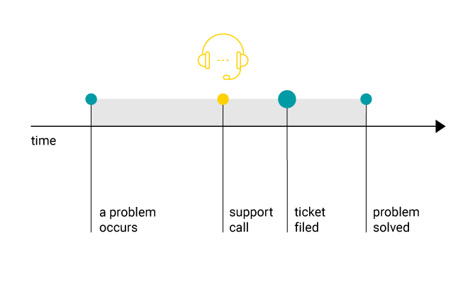
The complications stem from the fact we only have indirect information on the “goodness” state of the line (see diagram above). To construct a predictive model we need a labeled training set. Ideally, we would classify the interval between the occurrence of the problem and its resolution as the “bad” state and all other points in time as “good.” However, the only thing we could observe was the moment when a support ticket was filed. The delay between when the problem starts and when the user reports it is unknown and highly variable. It is actually not certain whether the problem will be reported at all, as different people have different thresholds for what they consider a problem. Even the point at which the problem is solved is uncertain: we have observed that 20% of the tickets are reissued within 10 days. This suggests that frequently problems are not fixed on the first try.
Another problem to solve for traditional binary classifiers was how to map time series to a list of features. We either only used parameter values from one point in time directly as features or we took an interval and converted it using tsfresh. We tried using k-means clusters and shape-based features (KShape) as extra features, but it did not bring us any gains.
We also had to diverge from the classical approach when evaluating the results. Traditionally, when evaluating a classifier we’d get measures like precision and recall. For time series, however, we couldn’t consider model runs in isolation. As we didn’t know the true onset of the problem, we decided that a positive prediction at most 3 days before a ticket was filed was a “hit.” Within this interval the model would run 18 times – if at any time it predicted a problem, we counted the whole interval as a single success. As we didn’t know when exactly the problem was fixed either, we added a grace period after the ticket was filed where we didn’t run the model. When we registered a false positive, we started a 3-day window in which any additional false positives didn’t count towards the total.
-2.png) We need to count true negatives and false positives in a different way from true positives and false negatives.
We need to count true negatives and false positives in a different way from true positives and false negatives.
We used a random forest model operating on tsfresh-converted time intervals. Time points near the support tickets were used as positive training examples and time points far away from tickets as negative training examples. As there was much more of the latter, we sub-sampled them to create a balanced training set.
Anomaly detection
The other broad class of approaches is anomaly detection (or one-class classifiers). In contrast to binary classifiers, it does not classify samples into arbitrarily selected classes based on training data but finds anomalies – points in the data set which are unlike most others. Its most important advantage is that it doesn’t need a labeled training set. The downside is that you cannot specify what you want to find. The classifier returns everything that it finds “interesting,” so this approach is effective to the extent that the subset you seek is small and distinct from the rest of the data set.
We tested two anomaly detection algorithms: isolation forest and threshold-based outlier detection. Isolation forest is a more powerful algorithm, but outlier detection is more explainable.
Outlier detection
The simplest form of anomaly detection is outlier detection. It works on one parameter at a time, detecting values that are further from the trend line than some threshold. The data on which the outlier algorithms operate is usually preprocessed by a seasonal-trend decomposition algorithm (more on that below). After preprocessing, we find the central value of the time series and its variability. We then treat all values which fall too far below or above the estimated variability as outliers. For example, we can compute the mean value and standard deviation of parameter values and treat all values which are more than 3 standard deviations apart from the mean as outliers.
There are other, more advanced methods. First, median absolute deviation (MAD) can be used as a robust replacement for the standard deviation. Second, more advanced iterative methods like Grubb's test or generalized extreme studentized deviate can be used.
Seasonal-trend decomposition
Seasonal-trend decomposition is a preprocessing step usually required before applying outlier detection algorithms. It is a transformation of a time series into three components:
- smoothly increasing or decreasing trend;
- periodic seasonal component;
- residual – what is left after subtracting the above components from the signal.
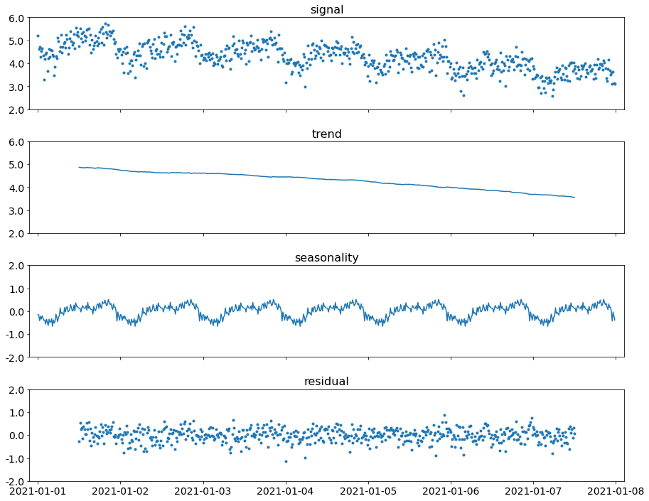
A signal being decomposed into a trend, seasonal component, and residual noise.
From the perspective of outlier detection, the decomposition removes predictable variability (trend and seasonality) from the signal, leaving only residual “noise.” Residuals are then easier to treat as if they were independent and distributed normally.
The simplest variant of decomposition uses a windowed moving average as the trend and the mean of parameter values at the same time of day as the seasonal component. Seasonal-trend decomposition using LOESS (STL) is a more advanced and computationally expensive alternative.
Practical decomposition algorithm implementations usually require equally spaced data. If data timing is variable, it can be converted by aggregation.
Isolation forest
The isolation forest is another anomaly detection method we tried. In contrast to outlier detection methods described above, it works on multi-dimensional data. Its downside is that it is not as easily explainable. Internally, it uses a set of isolation trees. This data structure is used to check whether a data point is far enough away from the majority of the points to be considered an outlier. Isolation forest has a parameter called contamination. Increasing its value increases the portion of the data set treated as anomalous.
We fed the isolation forest with all the data points independently. We did not preprocess the time series with tsfresh, so the classifier only considered the situation at one time point, without considering previous values of the parameter.
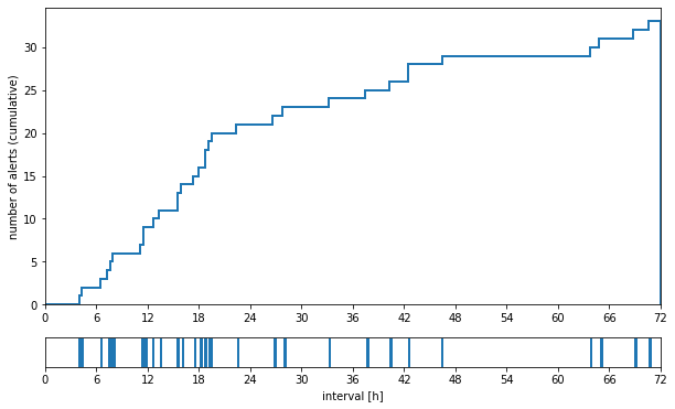
Time in hours from an alert being raised to a support ticket being filed, when predicted using the isolation forest. Most of the tickets are issued within one day from an alert being raised.
Results & future work
How useful a tool is, heavily depends on the context in which it is used. As said in the introduction, there are two scenarios against which we wanted to test our models: either before or after the end customer calls.
When it comes to predicting problems before they occur (i.e. before the call), there is still much to be done. As we’ve explained, only one in 2500 lines exhibits problems at any given moment, so the requirements for the specificity of the model are very stringent. A model which correctly recognizes lines without problems 99% of the time will still produce more false alarms than true ones. This is true even if it can correctly spot all real failures. In the plot below, you can see the performance of isolation forest and random forest models when used to predict support tickets.
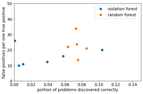
False positive to true positive ratio and recall of isolation forest and random forest models we constructed. In the case of random forest, each dot represents a run on a different subset of data. In the case of isolation forest, each dot represents a run with a different contamination parameter.
Because the majority of the lines were not broken, even a model with very high specificity would return a lot of false positives. Reducing the false positive rate to an acceptable level requires further research.
The results are much more optimistic and applicable for the other scenario: when the customer has already contacted the support. This is because the call in a way validates the prediction – when a customer reaches out, it’s more likely than not that the problem actually exists.
In order to help the customer center engineers troubleshoot problems, we need to consider another aspect: explainability, which will help us point them to the nature of the problem. On this front outlier detection takes the lead. Both random forest and isolation forest are complex models whose inner workings are not straightforward to explain. Meanwhile, detected outliers can be marked on the plot, showing both which parameters exceeded the threshold and when. Outlier detection models do not have as large a predictive power as other approaches we described, but they are explainable and do not need the training phase. This is why they are better if we want to provide customer care engineers with a graphical representation of anomalies when they are fixing issues.
Based on these observations, what conclusions do we have about the models we created?
- Both random forest and isolation forest models could reliably discover about 10% of support tickets. This was to be expected, as we only collected data related to the parameters of physical lines. There are other classes of problems, such as WiFi quality, which are undetectable from the data we used in this research. These will vary from one provider to another and further affect the results. This is why a comprehensive solution for forecasting customer issues requires data from other sources as well, starting with CPE monitoring and ending with business insights.
- Both models perform well when our goal is to provide guidance to the customer care engineer who is trying to solve a problem that’s already been reported. This is because, in this situation, we don’t need the extreme specificity required for predictive alerting. It may seem trivial at first, but being able to point to a possible problem with the physical line when the customer is calling both validates their claim (which is not always so obvious) and significantly narrows down the search. As we’ve pointed out above: there are many other reasons why the customer may have experienced problems. Identifying the source in the physical layer allows us to provide the operators with suggestions as to what steps they should take next to fix the problem.
This research provided us with valuable insights for future work on machine learning. In particular, it gave us a list of next steps to consider when working on tools for predictive alerting and customer support.
- Our samples were collected once every 4 hours, which makes it practically impossible to detect problems that were reported soon after they occurred. A way to potentially improve the prediction would then be to increase the sampling rate.
- As we’ve hinted above, we have discovered that tickets are frequently reissued within a few days for the same line, suggesting that the reparative actions taken were not really so reparative. For that data set, the number of “broken” and “not broken” devices is comparable, suggesting that the number of false alarms would be respectively smaller. In such a case, we can provide predictive alerts for ticket reissuing.
- One possible way to reduce the rate of false positives is to group lines that are physically connected to the same device (e.g. to the same DSLAM) and have the model only raise alerts if it detects problems on multiple lines within the same group. This is because, in a sense, the occurrence of multiple problems that have a common factor reinforces the presumption that the issue is on the side of the device they are connected by, rather than anything else.
- Instead of focusing on pinpointing issues, we can focus on an additional classification to find major classes of problems. This would allow us to point the engineers to the likely causes and fixes they can perform to resolve the issue. Again, this would be a step towards automatizing the whole process.